Tutorial: Querx in the spreadsheet
Automatically import and visualize recorded sensor values with LibreOffice Calc
Querx stores your measured values on the device and displays them graphically in the integrated web interface. In addition, there are various cloud and monitoring solutions for external data processing.
There is also the possibility to import measured values via the local network directly into your spreadsheet application for further processing. This enables the integration of Querx into existing processes, which are based on spreadsheets for many users.
This tutorial demonstrates this possibility by means of a Querx WLAN TH, whose measurement data is loaded into the open source and free program LibreOffice Calc for further processing and visualization.
Configuring the data import
First off, Calc shall be configured to request a dataset from the Querx device by (periodically) calling a certain URL and then copy the returned data into a spreadsheet.
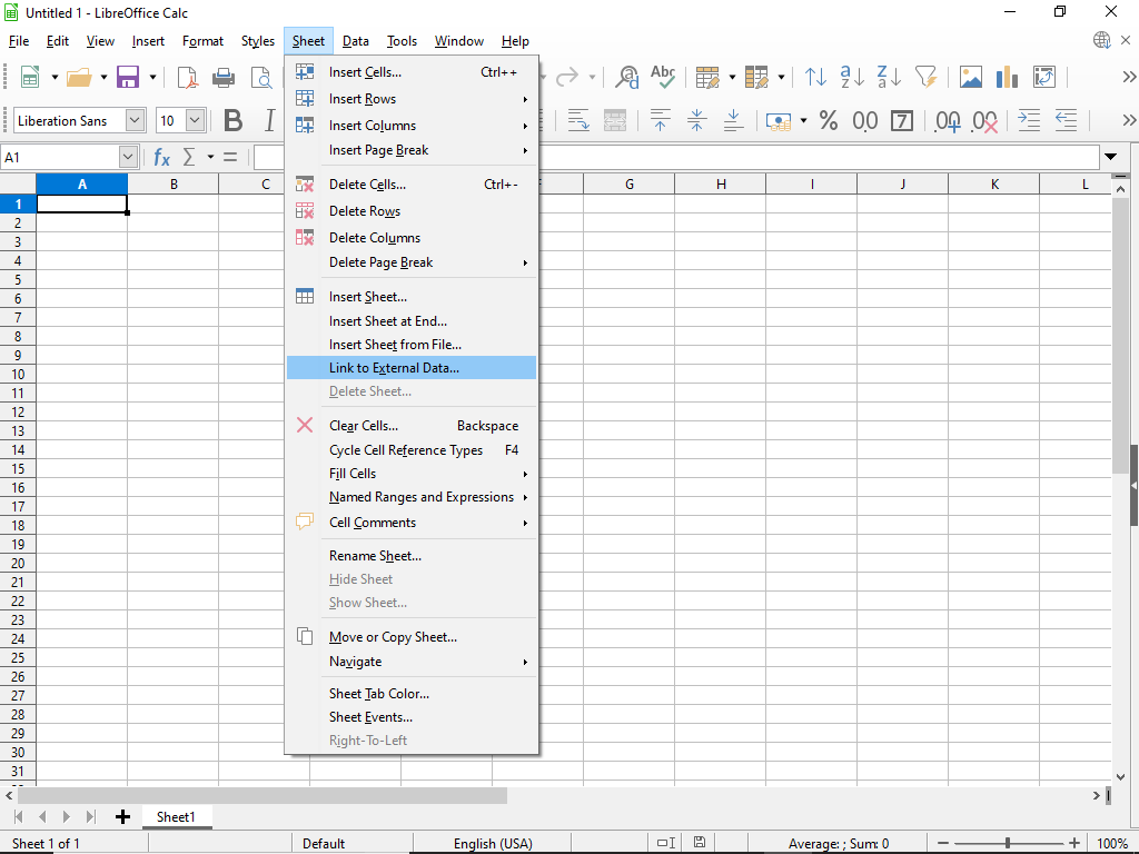
After you have created a new spreadsheet, select cell A1. This marks the position where the data should be inserted later.
Now click the menu item Link to External Data... in the Sheet menu.
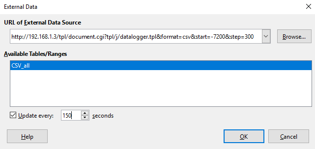
In the dialog window that opens, please insert the following URL into the field URL of External Data Source. Querx-IP must be replaced by the actual IP address of your device.
http://Querx-IP/tpl/document.cgi?tpl/j/datalogger.tpl&format=csv&start=-7200&step=300
This URL contains a number of parameters that determine how the data should be retrieved. In our example, the recorded measurement data should be requested in
- in CSV format (format=csv),
- from the current time, for the last 7200 seconds, that is two hours (start=-7200),
- with a step size of 300 seconds, i.e. 5 minutes (step=300).
In the Querx manual you will find a detailed explanation of all possible parameters in the chapter The HTTP Interface / Exporting Logged Data, which may be helpful, if you plan to realise your own requirements after this tutorial.

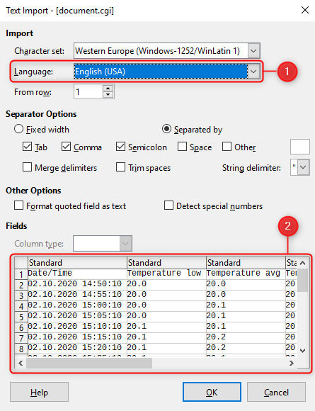
After you have entered the URL, press Enter while the focus is still on the URL input field. Another dialog window Text Import opens, which contains some settings and a preview 2 for the data import. The default settings can be kept, but please make sure, that in the selection menu Language English (USA) 1 is selected. This is necessary because the imported CSV document of Querx uses points as decimal separator for the measured values. The setting English (USA) ensures that Calc interprets these values correctly as decimal numbers, regardless of the locale settings of the application itself or your computer.
If your default settings should differ, please refer to the screenshot.
If you do not see a data preview in the lower part of the window, the import did not work. Check the URL (including the correct IP address of your Querx). To better isolate a possible issue, you can also try to access the URL with a web browser. If successful, you should receive a CSV file as an answer directly in the browser, or as a download.
If you see the preview data, click on OK.
In the dialog box beneath, activate the Update every: checkbox and enter 150 in the number field. This setting ensures that the data request is repeated every 150 seconds and our table will be automatically and periodically filled with up-to-date data.
Click on OK.
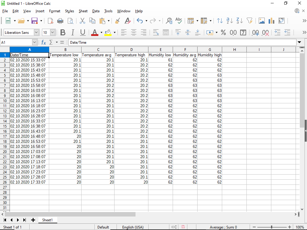
You should now see the imported readings in the spreadsheet. Because we have requested a time span of two hours and a step size of 5 minutes, the imported readings will have 25 rows. After 150 seconds you should also be able to see how the data gets automatically replaced by an updated version.
If you want to change the URL or its parameters, on the Edit menu, click on Links to External Files and then, in the dialog box that opens, double-click on the document.cgi line.

Further processing of the imported data: Dew point calculation
Now, as an example for the further use of the data, the dew point is to be calculated from the existing temperature and humidity values for the entire period. Thereby, measurement data of a Querx TH device is assumed. Querx PT devices do not measure humidity and are therefore unsuitable. If you are using a Querx THP, please note that three additional columns for the air pressure are added and the cell positions would change accordingly.
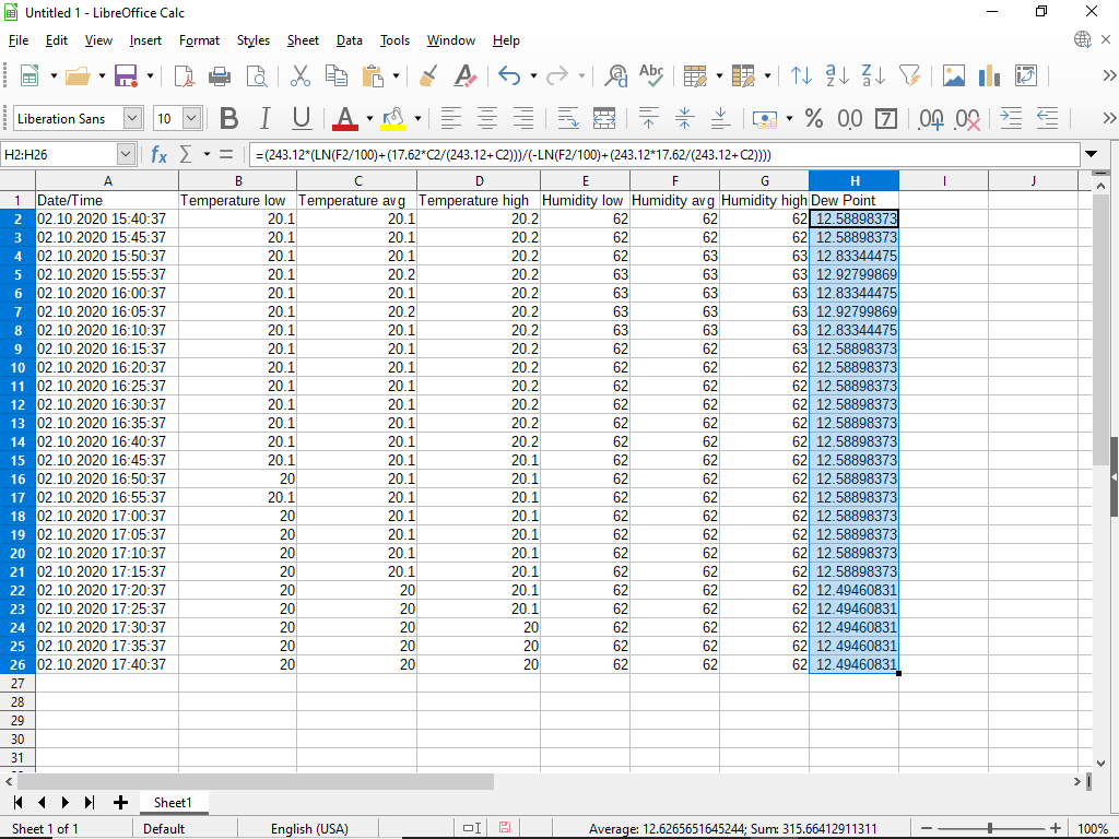
Select cell H1 and enter "Dew Point" as the column header.
To calculate the dew point at a given time, we use the formula for the dependence of dew point temperature on relative humidity and air temperature, using the average temperature (Temperature avg, column C) and the average relative humidity (Humidity avg, column F).
Now select cell H2 and insert the following formula (including the equals sign).
=(243.12*(LN(F2/100)+(17.62*C2/(243.12+C2)))/(-LN(F2/100)+(243.12*17.62/(243.12+C2))))
After pressing Enter, the calculated numerical value for the dew point of row 2 should appear in cell H2. Select the cell again and click on the black square at the bottom right-hand corner of the cell and drag the mouse down until all the cells in column H up to and including row 26 are marked with the purple frame. Now the complete column H should be filled with dew point values. From now on these values will also be updated automatically as soon as the program receives new data from Querx.
Visualization of the measured data
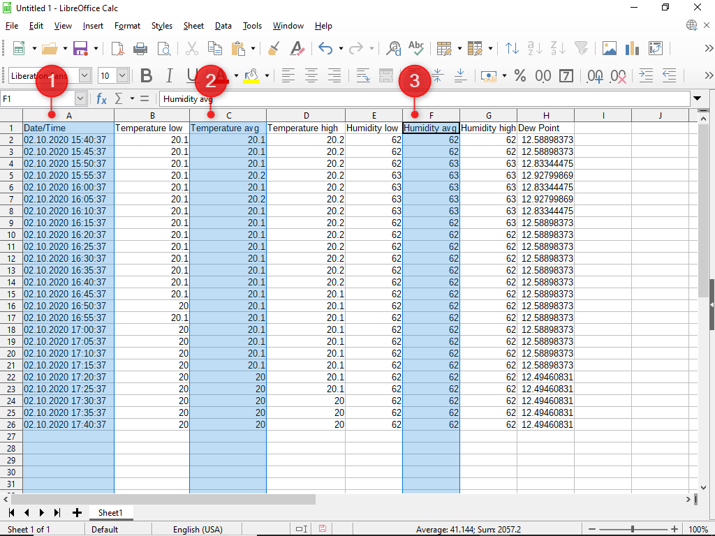
Finally, the measurement data shall be displayed in a line diagram. As an example, the average temperature (column C) and the average humidity (column F) over time (column A) are to be plotted.
Hold down the Ctrl key and click on the column titles A 1, C 2 and F 3. The selection should now look like the screenshot.
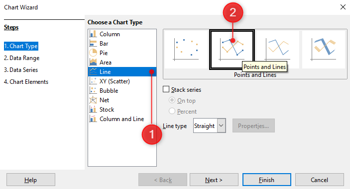
Select Chart from the Insert menu. In the Chart Wizard window, select Line, then Points and Lines.
Click on Exit.
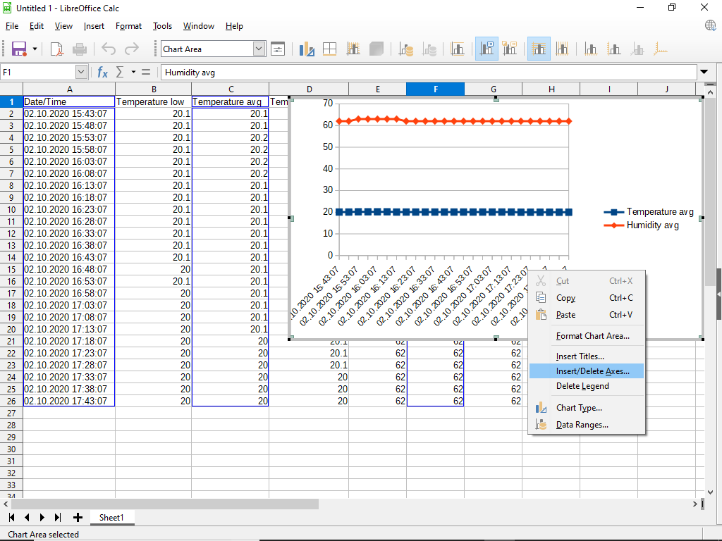
You should now see the line chart as in the screenshot. The diagram will be also updated automatically as soon as new measurement values arrive.
Currently both data series are related to a common axis. In the following, a secondary Y-axis is to be created and the humidity data series assigned to this axis. To do this, click with the right mouse button on the chart area and select Insert/Delete Axes... .
Then activate the check mark for Y-axis under Secondary Axes and confirm with OK.

Now select the data series for Humidity avg in the chart, click on it with the right mouse button and select Format Data Series... from the context menu. (You may have to double-click the chart area before you can select the data series).

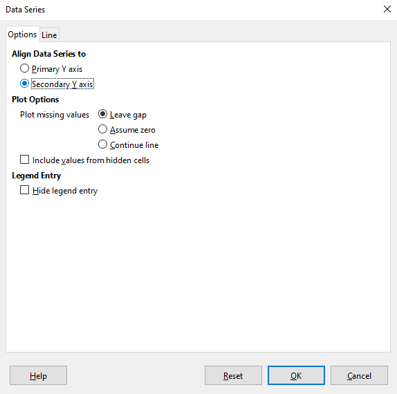
In the Options tab of the dialog box that opens, select the Secondary Y axis option under Align Data Series to and confirm with OK.
Done! Both data series should now use their own axes.

Many thanks to our community member Marco T. for the idea for this tutorial!